Squeeze-and-Excitation Block (SE Block)
[Reference]
논문 링크: Squeeze-and-Excitation Networks
- 2018년 (Arxiv)
- Jie Hu, Li Shen, Samuel Albanie, Gang Sun, Enhua Wu
- ILSVRC 2017 1st
Blog: https://inhovation97.tistory.com/48
목차
요약
- Squeeze Operation: 전체정보를 요약
- Excitation Operation: Squeeze Operation을 통해 계산된 Feature map의 중요도를 각 Channel에 곱해줌
- Squeeze, Excitation Operation을 통해 Representation power가 높은 Feature map에 Attention 할 수 있음
- 기존 VGG, GoogLeNet, ResNet 등 다양한 Network에 부착가능
- 기존 모델들에 SE Block을 결합시키면 Parameter가 크게 증가하지 않고, 높은 성능 향상
용어 정리
아래 네트워크 설명에 앞서, 등장하는 용어에 대한 간단한 설명
Excitation: 재조정
Global Average Pooling(GAP): Image의 모든 값의 평균을 구해 하나의 값으로 만듦

Convolution Operation: 1-1-Standard-Convolution 참고
Spatial: 공간 / x, y축과 같은 공간을 의미
Recalibration: 재조정
Bottleneck: 병목구조를 만들어 정보를 압축 (Embedding)
Skip Connection: Residual하게 연산된 값에 원본을 더하는 것 / 3-Inverted Residual 항목 참고
Local receptive field: 국부 수용영역 / 출력 뉴런 하나에 영향을 주고있는 입력 뉴런들 집합의 크기
빨간상의, 파란하의를 입고있는 사람의 이미지를 생각했을때,
어떤 Feature Map은 빨간 상의 영역의 가중치가 높고,
어떤 Feature Map은 파란 하의 영역의 가중치가 높고,
어떤 Feature Map은 배경 영역의 가중치가 높음
이때 각각의 Feature Map들은 저마다의 Local Receptive Field를 가지고 있다고 표현
설명
1. Other Network
SE Block이 시작되기전 다른 네트워크에 대한 부분.
그림과 같이 Convolution Operation가 있을수도 있고, GoogLeNet, VGGNet 등 다양한 Network가 올 수 있음
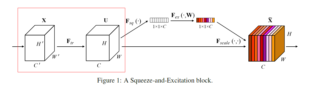
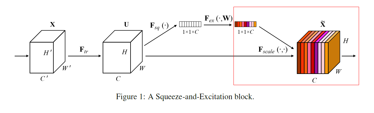
2. Squeeze Operation
Global Average Pooling을 통하여
의 이미지를 로 압축. 채널 개수만큼 연산 진행
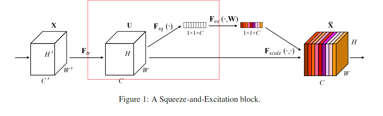
각 Channel을 대표하는 정보를 짜내는(Squeeze) 연산을 진행
- Feature Map들은 Local하게 생김
- 따라서 각 Feature Map들을 통해 Convolution Operation된 Image들은 각각 지역적인 정보만 가지고 있음 (= local receptive field)
- 여기서 우린, 지역적인 정보만이 아닌 전체적인 정보를 이용하고 싶음
- 전체적인 정보를 파악하기 전에, 각 지역적인 정보들의 대표값들을 Squeeze해서 구해놓는 단계
- Feature Map(=filter)는 Receptive Field가 Local 하기 때문에, Global한 관점에서 Contextual(문맥적인) 정보를 이용할 수 없음
- Squeeze Operation 단계는 Local receptive field 밖의 정보를 이용하기 전에
(Global Spatial Information)의 image를 각 채널별로 Squeeze하여 Channel Descriptor(각 채널을 가장 잘 설명하는 값으로) 제작
Squeeze Operation을 나타내는 수식
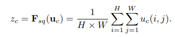
연산은 용어 정리 파트에 기술한대로 각 Channel의 크기의 Global Spatial Information을 로 압축하는 연산
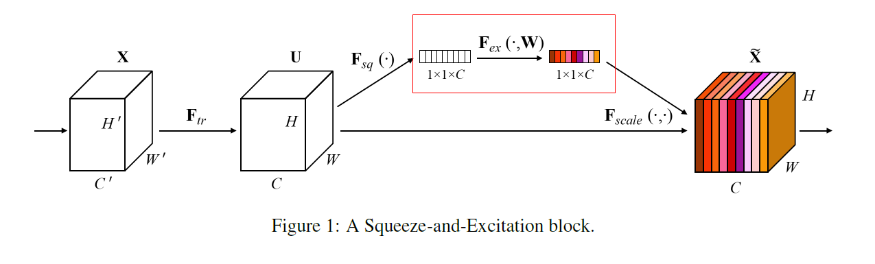
3. Excitation Operation
Squeeze Operation을 통해 각 채널들을 대표하는 값들을 얻었고, 이제 이 값들을 이용하여 문맥적인(Contextual) 정보를 얻기위해 Excitation Operation 진행
Channel 간의 상호작용(또는 의존성)을 학습하기 위해 다음의 두 가지 조건이 충족되어야 함
Flexible 해야함
이 말은 곧, 채널들간 Non-linear한 특성을 파악할 수 있어야함
Non-mutually-exclusive한 관계를 학습해야함
전체적인 맥락파악을 위해 한개의 채널만 강조(one-hot activation)되면 안되고, 다양한 채널들이 강조되어야함
Excitation Operation을 나타내는 수식

는 Fully Connected Layer에서 곱해지는 가중치행렬을 의미 는 ReLU Activation Operation을 의미 는 Sigmoid Activation Function을 의미 - 3-1-Gating Mechanism에서 이어서 설명
3-1. Gating Mechanism
위에 설명된 조건을 충족하기 위해 제작됨
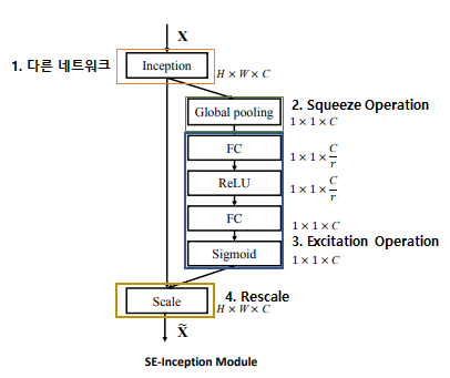
두개의 Fully Connected Layer로 Bottleneck 형성
FC1에서 Reduction Ratio(
)을 이용하여, 채널의 수를 에서 로 압축 ReLU 을 통해 비선형성 부여
FC2에서 다시 Channel의 수를
에서 로 확장 압축하고 팽창하는 과정을 통해 모델의 복잡도를 제한하고, 정보를 일반화 함
Sigmoid를 통해 모든 값들을 0~1 사이의 값으로 정규화시켜, 채널의 중요도를 표현하게 함
4. Rescaling
3-Excitation Operation을 통해 최종적으로 출력된 각 Channel별 중요도 값을 기존의 이미지행렬(
)의 각 채널에 곱하는 작업
Self-Attention
- Local한 각 채널들의 정보들을 이용하여 채널간의 관계들을 파악하고, 채널들의 중요도로 표현하여 기존 Image 행렬에 적용
- 전체적인 맥락을 고려하여 그때그때 상황에 맞는 Channel을 강조함
5. Model and Computational Complexity
SE Block 역시 Performance와 Model Complexity의 Trade-off가 있지만, 굉장히 작다
추가되는 파라미터는 다음과 같음
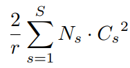
: Reduction ratio : Number of stages / 단계(Squeeze, FC layer1, FC layer2, ...) : Dimension of the output channels : Repeated block number for stage SE block을 적용시킨 SE-ResNet-50의 경우
기존 ~25 Million Parameters를 가지고 있던 ResNet-50에서 ~2.5 million의 Additional Parameters가 추가됨
약 10% 정도의 Computational Cost 증가
마지막 Layer에 부착된 SEBlock은 제거해도 성능엔 큰 영향을 미치지 않으면서(top-5 error < 0.1% 증가), 연산량은 ~4% 감소시킴
이미 다양한 Layer와 SEBlock들을 통과해오며, 각 Feature의 전문가들이 되어있어 Channel별 정보교환이 의미가 적음
Reduction ratio
에 따른 영향은 다음과 같음 이어도 Error에는 큰 영향을 미치지 않으며 에 비해 38%의 Parameter 감소효과가 있음 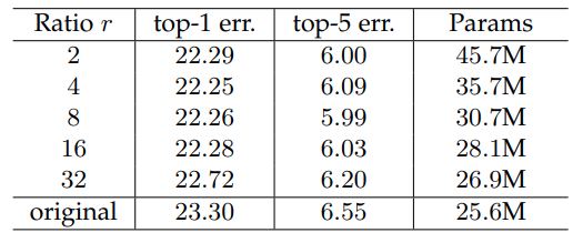
SEBlock을 MobileNet과 ShuffleNet에 적용시킨 경우
Re-implementation과 SENet을 적용시킨 것을 비교해봤을때 MobileNet에서 Params
증가, error ~3.1%까지 감소

구현
[Code Reference]
1. 코드 개요
Dataset은 TorchVision에서 제공하고있는 STL10 Dataset 이용
- Train: 5000개 / Test: 8000개
- airplane, bird, car, cat, deer, dog, horse, monkey, ship, truck 항목에 대한 Dataset
3-1. Gating Mechanism을 설명하기위한 그림의 1번 "다른 네트워크"를 MobileNetV1의 Separable Depthwise Convolution 연산으로 대체
- Depthwise Conv - Pointwise Conv - SEBlock으로 구성하여 학습
총 3가지의 파일
- SEBlock.py: Separable Depthwise Convolution Block 하단에 SEBlock 붙여서 구현
- SEBlock_train.py: STL10 Data 전처리 및 학습진행
- SEBlock_inference.py: 학습된 모델을 이용하여 추론
2. 코드
자세한 설명은 주석 설명 또는 Reference블로그 참고
2-1. SEBlock.py
import torch
import torch.nn as nn
import torch.nn.functional as F
from torch import optim

from torchvision import datasets
from torch.utils.data import DataLoader

from torchvision import utils
import matplotlib.pyplot as plt

import numpy as np
from torchsummary import summary
import time
import copy
import os

class SEBlock(nn.Module):
    def __init__(self, in_channels, r=16):
        super(SEBlock, self).__init__()

        # 본문 2번항목: Squeeze Operation
        self.squeeze = nn.AdaptiveAvgPool2d((1, 1))
        # 본문 3번 항목: Excitation Operation
        self.excitation = nn.Sequential(
            nn.Linear(in_channels, in_channels // r),
            nn.ReLU(),
            nn.Linear(in_channels // r, in_channels),
            nn.Sigmoid()
        )

    def forward(self, x):
        x = self.squeeze(x) # Global Average Pooling
        x = x.view(x.size(0), -1)   # Batch size축은 놔두고 나머지를 일렬로 쭉 펴기
        x = self.excitation(x)
        x = x.view(x.size(0), x.size(1), 1, 1)  # 원래대로 복구
        return x


# MobileNetV1을 구현하기위한
# Separatable Depthwise Convolution 블록 구현
class Depthwise(nn.Module):
    def __init__(self, in_channels, out_channels, stride=1):
        super(Depthwise, self).__init__()
        self.depthwise = nn.Sequential(
            nn.Conv2d(in_channels, in_channels, kernel_size=3, stride=stride, padding=1, groups=in_channels, bias=False),
            nn.BatchNorm2d(in_channels),
            nn.ReLU6(),
        )

        self.pointwise = nn.Sequential(
            nn.Conv2d(in_channels, out_channels, kernel_size=1, stride=1, padding=0, bias=False),
            nn.BatchNorm2d(out_channels),
            nn.ReLU6()
        )

        # Separable Depthwise Convolution의 마지막 부분에 SEBlock 붙임
        self.seblock = SEBlock(out_channels)

    def forward(self, x):
        x = self.depthwise(x)
        x = self.pointwise(x)
        x = self.seblock(x) * x # 본문 4번 항목: Scailing
        return x

class BasicConv2d(nn.Module):
    def __init__(self, in_channels, out_channels, kernel_size, **kwargs):
        super(BasicConv2d, self).__init__()
        self.conv = nn.Sequential(
            nn.Conv2d(in_channels, out_channels, kernel_size=kernel_size, **kwargs),
            nn.BatchNorm2d(out_channels),
            nn.ReLU6()
        )

    def forward(self, x):
        x = self.conv(x)
        return x

# MobileNetV1
class MobileNetV1(nn.Module):
    def __init__(self, width_multiplier, num_classes=10, init_weights=True):
        super().__init__()
        self.init_weights=init_weights
        alpha = width_multiplier

        self.conv1 = BasicConv2d(3, int(32*alpha), int(64*alpha), stride=1)
        self.conv2 = Depthwise(int(32*alpha), int(64*alpha), stride=1)

        # 이미지 크기 반으로 줄이고, Channel 증가 시키기
        self.conv3 = nn.Sequential(
            Depthwise(int(64*alpha), int(128*alpha), stride=2),
            Depthwise(int(128*alpha), int(128*alpha), stride=1)
        )
        self.conv4 = nn.Sequential(
            Depthwise(int(128*alpha), int(256*alpha), stride=2),
            Depthwise(int(256*alpha), int(256*alpha), stride=1)
        )
        self.conv5 = nn.Sequential(
            Depthwise(int(256*alpha), int(512*alpha), stride=2),
            Depthwise(int(512*alpha), int(512*alpha), stride=1),
            Depthwise(int(512*alpha), int(512*alpha), stride=1),
            Depthwise(int(512*alpha), int(512*alpha), stride=1),
            Depthwise(int(512*alpha), int(512*alpha), stride=1),
            Depthwise(int(512*alpha), int(512*alpha), stride=1),
        )
        self.conv6 = nn.Sequential(
            Depthwise(int(512*alpha), int(1024*alpha), stride=2)
        )
        self.conv7 = nn.Sequential(
            Depthwise(int(1024*alpha), int(1024*alpha), stride=2)
        )

        # 추론 파트
        self.avg_pool = nn.AdaptiveAvgPool2d((1, 1))
        self.linear = nn.Linear(int(1024*alpha), num_classes)

        # weight 초기화
        if self.init_weights:
            self._initialize_weights()

    def forward(self, x):
        x = self.conv1(x)
        x = self.conv2(x)
        x = self.conv3(x)
        x = self.conv4(x)
        x = self.conv5(x)
        x = self.conv6(x)
        x = self.conv7(x)
        x = self.avg_pool(x)
        x = x.view(x.size(0), -1)
        x = self.linear(x)
        return x

    def _initialize_weights(self):
        for m in self.modules():
            if isinstance(m, nn.Conv2d):
                nn.init.kaiming_normal_(m.weight, mode='fan_out', nonlinearity='relu')
                if m.bias is not None:
                    nn.init.constant_(m.bias, 0)
            elif isinstance(m, nn.BatchNorm2d):
                nn.init.constant_(m.weight, 1)
                nn.init.constant_(m.bias, 0)
            elif isinstance(m, nn.Linear):
                nn.init.normal_(m.weight, 0, 0.01)
                nn.init.constant_(m.bias, 0)

def mobilenetv1(alpha=1, num_classes=10):
    return MobileNetV1(alpha, num_classes)


if __name__ == "__main__":
    device = torch.device('cuda' if torch.cuda.is_available() else 'cpu')

    x = torch.randn(3, 3, 224, 224).to(device)
    model = mobilenetv1().to(device)
    output = model(x)
    print(output.size())
    summary(model, (3, 224, 224))
2-2. SEBlock_train.py
from matplotlib.style import available
import torch
import torch.nn as nn
import torch.nn.functional as F
from torchsummary import summary
from torch import optim

# dataset and transformation
from torchvision import datasets
import torchvision.transforms as transforms
from torch.utils.data import DataLoader
import os

# display images
from torchvision import utils
import matplotlib.pyplot as plt

# utils
import numpy as np
from torchsummary import summary
import time
import copy

from SEBlock import mobilenetv1

# weight 저장할 디렉토리 확인 후 없으면 제작
def createFolder(directory):
    try:
        if not os.path.exists(directory):
            os.makedirs(directory)
    except OSError:
        print('Error')

device = torch.device('cuda' if torch.cuda.is_available() else 'cpu')

data_path = './data'
if not os.path.exists(data_path):
    os.mkdir(data_path)


# 데이터셋 불러오기
train_ds = datasets.STL10(data_path, split='train', download=True, transform=transforms.ToTensor())
val_ds = datasets.STL10(data_path, split='test', download=True, transform=transforms.ToTensor())

transformation = transforms.Compose([
    transforms.ToTensor(),
    transforms.Resize(224)
])

# 데이터 변형 (이미지 리사이즈)
train_ds.transform = transformation
val_ds.transform = transformation

# 데이터로더에 올리기
train_dl = DataLoader(train_ds, batch_size=32, shuffle=True)
val_dl = DataLoader(val_ds, batch_size=32, shuffle=True)

# Loss와 Optimizer 설정
model = mobilenetv1().to(device)
loss_func = nn.CrossEntropyLoss(reduction='sum')    # 나온 loss값들 다 더해서 알려줌
opt = optim.Adam(model.parameters(), lr=0.01)

from torch.optim.lr_scheduler import ReduceLROnPlateau
lr_scheduler = ReduceLROnPlateau(opt, mode='min', factor=0.1, patience=10)  # 모델의 개선이 없을 경우 Learning Rate를 조절하여 개선을 유도
"""
# opt: 조절의 기준이 되는 값
# mode: 'min' 최소가 될수있도록 수정
# factor: 계수
# patience: Patience 만큼의 Epoch동안 개선이 없으면 수정
"""

createFolder('./models')
# Training 파라미터 설정
params_train = {
    'num_epochs':100,
    'optimizer':opt,
    'loss_func':loss_func,
    'train_dl':train_dl,
    'val_dl':val_dl,
    'sanity_check':False,
    'lr_scheduler':lr_scheduler,
    'weight_path':'./models/weights.pt',
}


def show(img, y=None):
    npimg = img.numpy()
    npimg_tr = np.transpose(npimg, (1, 2, 0))   # (3, 228, 228) 형태의 이미지를 (228, 228, 3)형태로 바꾸어서 plt로 표현 가능하게 변경
    plt.imshow(npimg_tr)

    if y is not None:
        plt.title('labels:' + str(y))

# 현재의 Learning Rate 리턴
def get_lr(opt):
    for param_group in opt.param_groups:
        return param_group['lr']

# mini-batch당 metric 계산
def metric_batch(output, target):
    pred = output.argmax(1, keepdim=True)
    corrects = pred.eq(target.view_as(pred)).sum().item()   # pred와 target의 일치 개수 더해서 리턴
    return corrects

# mini-batch당 loss 계산
def loss_batch(loss_func, output, target, opt=None):
    loss_b = loss_func(output, target)
    metric_b = metric_batch(output, target)

    if opt is not None:
        opt.zero_grad() # 계산할때마다 opt 초기화해줘야함
        loss_b.backward() # Back propagation으로 loss 계산
        opt.step()  # weight에 적용

    return loss_b.item(), metric_b  # loss와 correct값 구해서 리턴

# epoch별로 loss 구하기
def loss_epoch(model, loss_func, dataset_dl, opt=None):
    running_loss = 0.0
    running_metric = 0.0
    len_data = len(dataset_dl.dataset)

    # DataLoader를 통해 Data를 Batch단위로 빼옴
    for xb, yb in dataset_dl:
        xb = xb.to(device)  # data를 device에 올리기
        yb = yb.to(device)  # label도 device에 올리기
        output = model(xb)

        # Batch 단위로 Loss와 Correct 계산
        loss_b, metric_b = loss_batch(loss_func, output, yb, opt)

        running_loss += loss_b

        if metric_b is not None:
            running_metric += metric_b

    loss = running_loss / len_data
    metric = running_metric / len_data
    return loss, metric

# Train Part
def train(model, params):
    num_epochs=params['num_epochs']
    loss_func=params['loss_func']
    opt=params['optimizer']
    train_dl=params['train_dl']
    val_dl=params['val_dl']
    lr_scheduler=params['lr_scheduler']
    weight_path=params['weight_path']

    loss_history = {'train': [], 'val': []}
    metric_history = {'train': [], 'val': []}

    best_loss = float('inf')
    best_model_wts = copy.deepcopy(model.state_dict())
    start_time = time.time()

    for epoch in range(num_epochs):
        current_lr = get_lr(opt)
        print('Epoch {}/{}, current lr= {}'.format(epoch, num_epochs-1, current_lr))

        model.train()
        train_loss, train_metric = loss_epoch(model, loss_func, train_dl, opt)
        loss_history['train'].append(train_loss)
        metric_history['train'].append(train_metric)

        model.eval()
        with torch.no_grad():
            val_loss, val_metric = loss_epoch(model, loss_func, val_dl)
        loss_history['val'].append(val_loss)
        metric_history['val'].append(val_metric)

        if val_loss < best_loss:
            best_loss = val_loss
            best_model_wts = copy.deepcopy(model.state_dict())
            torch.save(model.state_dict(), weight_path)
            print('Copied best model weights!')

        lr_scheduler.step(val_loss)
        if current_lr != get_lr(opt):
            print('Loading best model weights!')
            model.load_state_dict(best_model_wts)

        print('train loss: %.6f, val loss: %.6f, accuracy: %.2f, time: %.4f min' %(train_loss, val_loss, 100*val_metric, (time.time()-start_time)/60))
        print('-'*10)

    model.load_state_dict(best_model_wts)
    return model, loss_history, metric_history


if __name__ == "__main__":
    model, loss_hist, metric_hist = train(model, params_train)
2-3. SEBlock_inference.py
from matplotlib.style import available
import torch
import torch.nn as nn
import torch.nn.functional as F
from torchsummary import summary
from torch import optim
# dataset and transformation
from torchvision import datasets
import torchvision.transforms as transforms
from torch.utils.data import DataLoader
import os
# display images
from torchvision import utils
import matplotlib.pyplot as plt
# utils
import numpy as np
from torchsummary import summary
import time
import copy
from SEBlock import mobilenetv1
def show(img, y=None):
npimg = img.numpy()
npimg_tr = np.transpose(npimg, (1, 2, 0)) # (3, 228, 228) 형태의 이미지를 (228, 228, 3)형태로 바꾸어서 plt로 표현 가능하게 변경
plt.imshow(npimg_tr)
if y is not None:
plt.title('labels:' + str(y))
plt.pause(0.001)
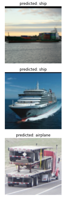
def visualize_model(model, num_images=10):
was_training = False
model.eval()
images_so_far = 0
with torch.no_grad():
print(3)
for data in val_dl:
images, labels = data
images = images.to(device)
labels = labels.to(device)
outputs = model(images)
_, predicted = torch.max(outputs.data, 1)
for j in range(images.size()[0]): # 배치 사이즈 만큼 넣음
images_so_far += 1
plt.figure(figsize=(20, 20))
ax = plt.subplot(num_images//2, 2, images_so_far)
ax.axis('off')
ax.set_title('predicted: {}'.format(classes[predicted[j]])) # 예측한 애들을 이제 Class 명으로 변환
show(images.cpu().data[j])
if images_so_far == num_images:
model.train(mode=was_training) # model.train(mode=False) == model.eval()
return
model.train(mode=was_training)
if __name__ == "__main__":
device = torch.device('cuda' if torch.cuda.is_available() else 'cpu')
data_path = './data'
weight_path = './models/weights.pt'
classes = (
'airplane',
'bird',
'car',
'cat',
'deer',
'dog',
'horse',
'monkey',
'ship',
'truck'
)
train_ds = datasets.STL10(data_path, split='train', download=True, transform=transforms.ToTensor())
val_ds = datasets.STL10(data_path, split='test', download=True, transform=transforms.ToTensor())
transformation = transforms.Compose([
transforms.Resize((224, 224)),
transforms.ToTensor()
])
# 데이터셋 준비 완료
train_ds.transform = transformation
val_ds.transform = transformation
# 데이터로더에 배치로 올리기
train_dl = DataLoader(train_ds, batch_size=32, shuffle=True)
val_dl = DataLoader(val_ds, batch_size=32, shuffle=True)
# 모델 불러오기
model = mobilenetv1().to(device)
print(1)
checkpoint = torch.load(weight_path)
model.load_state_dict(checkpoint)
print(2)
# 모델 추론 및 시각화
visualize_model(model)
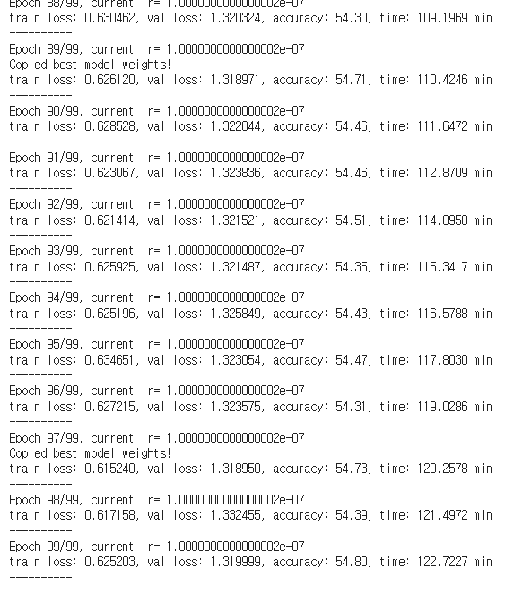
3. 결과
MobileNetV1 + SEBlock
- 100 epoch 동안 54.80%의 Accuracy 달성
- STL10 Dataset에는 Label이 없는 Dataset이 많음(10만개) 따라서 더 많은 Epoch를 돌리거나
- learning rate scheduler를 Cosine Annealing을 사용했을 때, 성능향상 기대
'Computer Vision' 카테고리의 다른 글
| NAFNet 쉬운 논문 리뷰 (0) | 2022.11.27 |
|---|---|
| MobileNetV3 쉬운 논문 리뷰 및 Pytorch 구현 (0) | 2022.08.02 |
| MnasNet 쉬운 논문 리뷰 (0) | 2022.08.01 |
| ShuffleNet 쉬운 논문 리뷰/구현 (0) | 2022.07.20 |
| MobileNet V2 쉬운 논문 리뷰/구현 (1) | 2022.07.07 |


댓글